The ML Production Readiness of Tesla’s Autopilot

Read this post on Medium.

Disclaimer: I previously interned at Tesla on things unrelated to Autopilot, and I now work at Google, where I am compensated in part through Alphabet stock. I do not own any Tesla stock. Below are my personal views, not those of either company.


Many companies are scrambling to deploy ML and “AI” in their products, either to be genuinely innovative or at least to appear so. Like most other software, ML models are prone to bugginess and failure, although oftentimes in new and unexpected ways. In conventional software development, we test code to preemptively catch the kind of faults one might encounter in production and give some assurances of correctness. In ML model development, the best ways to test ML for production readiness are still fairly new and are often domain-specific.

More worryingly, very few companies test their ML models and code at all — simply “doing ML” is seen as enough. In conventional software development, having bugs in production services can lead to a negative user experience and lost revenue. Since ML models are being put to work widely in the real world and the failures are often more subtle, the overall effects can be more harmful. For an e-commerce company, a buggy model can lead to poor product recommendations. For a self-driving car company, a buggy model can lead to people dying.

The goal of this post is to assess how current ML production best practices might apply to the development of a self-driving car, and where Tesla’s efforts in particular may be falling short. This isn’t mean to be a Tesla “hit piece” — Tesla is just one of many companies deploying self-driving cars with a cavalier attitude towards thoroughness and safety. In particular, they have the largest deployed fleet of semi-autonomous vehicles, and don’t mind using the words “beta” and “self-driving car software” in the same sentence.

The analysis below is based on the paper “The ML Test Score: A Rubric for ML Production Readiness and Technical Debt Reduction” and Andrej Karpathy’s recent talk, “Building the Software 2.0 Stack”. I recommend reading the entire paper and watching the entire talk if you have the time. The paper gives concrete steps a company can take to test ML models for production readiness, and the talk gives an honest look at some of the data-related challenges around building self-driving cars.

Data

Feature expectations are captured in a schema.

All features are beneficial.

No feature’s cost is too much.

Features adhere to meta-level requirements.

The data pipeline has appropriate privacy controls.

New features can be added quickly.

All input feature code is tested.

Karpathy’s talk focuses almost entirely on the collection and labelling of data as the main problem behind his team’s work. His reasoning is that where there were once engineers writing new algorithms for each task, there are now labellers generating high-quality data for predefined algorithms to learn each task from, so most ML problems are really just data problems.

Breck’s paper focuses on the practical aspects of testing data pipelines that feed models. These are standard software engineering best practices applied to data-ingestion techniques. We can’t assume what Tesla’s internal software engineering practices are like, but we can assert that any serious self-driving car program must have a robust data management operation, or it will not succeed.

Privacy is the only data principle that stands out as more than a mere technical detail. The idea of privacy controls applied to self-driving car data is a nascent area of study, though it has some precedent in Google’s Street View imagery. Some startups will gladly pay you in exchange for your driving data, but Tesla gets it for free from their fleet. They are at the very least asking for users’ permission to record video from their cars, though we can’t know whether or not the internal privacy controls on that data are satisfactory, and how they may or may not comply with GDPR. The privacy of those being recorded in public also comes into question — in this video from Cruise, for example, people’s faces are recorded and displayed without any anonymization.

Model Development

Model specs are reviewed and submitted.

Offline and online metrics correlate.

All hyperparameters have been tuned.

The impact of model staleness is known.

A simpler model is not better.

Model quality is sufficient on important data slices.

The model is tested for considerations of inclusion.

This section focuses on the process of model development itself. Though the Tesla Autopilot team likely spends a significant amount of effort on building and testing various models, Karpathy’s talk frames modeling as essentially a solved problem when compared to data collection. Indeed, current Autopilot versions appear to be using fairly standard architectures.

Still, model development has its nuances. Inference must be fast, so tradeoffs between performance and latency must be taken into account. Hyperparameter (or even architecture) tuning must be done to eek out any last remaining gains in performance on the desired data.

Model staleness in the case of self-driving cars is an interesting one. Consider, for example, the changing of the seasons. A model whose primary input is visual data would perform slightly differently in different weather conditions during different parts of the year, depending on the data coverage of those conditions. Since Tesla is a global company, ideally they would have coverage of all conditions in different areas and climates, and models would be tested on all available data.

The same ideas can be applied to inclusion — which types of roads and neighborhoods does Tesla have good training data for? Karpathy’s talk gets into the nuances of stop signs, road markers, inclines, and traffic lights in various parts of the world, so it is reasonable to expect that they’re testing their models on edge cases as much as possible and filling in the gaps in their datasets as soon as they appear.

Infrastructure

Training is reproducible.

Model specs are unit tested.

The ML pipeline is Integration tested.

Model quality is validated before serving.

The model is debuggable.

Models are canaried before serving.

Serving models can be rolled back.

Infrastructure tests are particularly interesting when applied to self-driving cars. In contrast to more conventional ML architectures, which are often served from centralized servers in data centers, self-driving cars do almost everything on the edge, in each individual car itself. As a result, a self-driving vehicle should have both hardware and software redundancy to be tolerant against failures. Tesla’s current lineup lacks hardware redundancy. Since software updates are delivered OTA, it is completely reasonable to expect that Tesla has mechanisms in place to allow Autopilot versions to be rolled back immediately in case there is an unexpected regression in performance, though such a rollback would still need to be triggered from some central source.

Tesla’s camera-centric hardware introduces its own set of problems. Considerations like white balance, color calibration, and various other sensor properties need to be consistent across data and devices, otherwise uncertainty can be introduced in both training and inference. Such differences can be especially pronounced in different lighting (daytime vs. nighttime) and weather conditions.

Additionally, simulation is an essential part of any robust self-driving car operation. Being able to test new iterations of models against all historical data is key to safe iteration that ensures there are no regressions for certain slices of the data. Simulation is especially important in such high-stakes scenarios when A/B testing in the real world isn’t an option. It’s unclear how much work Tesla is doing in the simulation space, though it’s likely not enough if we’re judging by their job postings.

Monitoring

Dependency changes result in notification.

Data invariants hold for inputs.

Training and serving are not skewed.

Models are not too stale.

Models are numerically stable.

Computing performance has not regressed.

Prediction quality has not regressed.

Monitoring a live system is especially important in ensuring that performance remains reliable as the system itself or the world around it change. In the case of Tesla’s vehicles, the hardware’s health would need to be monitored to detect any issues with cameras or other sensors, as well as the hardware that runs inference, as the components age. Any issues with other fundamental features of the car’s operating system can all affect the reliability of the parts of the system running model inference.

Model staleness that isn’t addressed through a varied enough dataset (for example, exceptionally smokey skies during a wildfire) would need to be addressed through regular OTA updates, which comes with its own set of infrastructure challenges. Again, because these systems are being run on the edge, Tesla has more control while creating and improving the model, but must provide failsafe guarantees when the model is deployed and out of their immediate control.

Conclusion

These are only a few of the most obvious concerns a company such as Tesla might encounter when building a reliable self-driving car, as viewed through the lens of building production ML systems for lower-stakes consumer software. Surely the Autopilot team has considered each of these scenarios, but considering them from the perspective of a battle-tested production ML checklist offers a helpful way of framing problems in better-understood domains to anticipate problems in this new one. From the simple analysis above, it seems that Tesla has a significant set of challenges to address before it can claim to have safe and reliable self-driving capabilities in its vehicles.

FAT* 2018 Conference Notes, Day 2

Keynote 2: Deborah Hellman

Deborah Hellman of UVA Law starts the day off with a keynote on justice and fairness. She opens with a quote from Sidney Morgenbesser about what is unfair and what is unjust, asking if fairness is about treating everyone the same. She follows with a quote from Anatole France — “In its majestic equality, the law forbids rich and poor alike to sleep under bridges, beg in the streets and steal loaves of bread.” In practice, policies that formally treat everyone the same affect people in different ways.

Hypothesis 1: Treat like cases alike.
This hypothesis relies on choosing a proxy by which to classify people and decide how to treat them differently. That is, if treating everyone the same is unfair because of the situations they’re in lead to different outcomes, classify them into different cases based on their situations, and treat each case separately. This hypothesis seems to fall apart based on how the classifications are made and the intentions of those classifications in search of certain outcomes. This leads to the next hypothesis…

Hypothesis 2: It’s the thought that counts.
These traits are usually adopted for bad reasons. The classifications are made to impose differing treatments with moral decisions that are misguided or unjust. For example, an employer may avoid hiring women between the ages of 25 and 40 to avoid having to pay women who may have children to take care of. The goal is not to avoid employing women, but to increase productivity. The intent behind the classification is itself misguided or flawed.

Hypothesis 3: “Anti-Classification”
The use of classifications, in particular classifications based on certain traits e.g. race, gender, can lead to unintended effects and denigration.

Hypothesis 4: Bad Effects
Certain classifications themselves can compound injustice — for example, charging higher life insurance rates to battered women.

Hypothesis 5: Expressing Denigration
For example, saying “All teengaers must sit in the back of the bus” vs. “All blacks must sit in the back of the bus” express different ideas. Regardless of the intention, there is denigration inherent in the classification. She cites Justice Harlan’s dissent in Plessy v. Ferguson.

Indirect Discrimination and the Duty to Avoid Compounding Injustice
The Empty Idea of Equality
Even Imperfect Algorithms Can Improve the Criminal Justice System

Discussion: Cynthia Dwork

Session 3: Fairness in Computer Vision and NLP

Gender Shades: Intersectional Accuracy Disparities in Commercial Gender Classification (data)

Joy Buolamwini gives a talk on her now infamous paper on the poor performance of facial analysis technologies on non-white, non-male faces. She uses a more diverse dataset to benchmark various APIs. After reporting the poor performance to various companies, some actually improved their models to account for the underrepresented classes.

See also:
The Perpetual Line-Up

Analyze, Detect and Remove Gender Stereotyping from Bollywood Movies

Taneea Agrawaal presents her analysis of gender stereotyping in Bollywood movies. The analysis was done with a database of Bollywood movies going back intio the 1940s, along with movie trailers from the last decade and a few released movie scripts. Syntax analysis is done to extract verbs related to males and females to study the actions associated with each. She argues that the stories told and representations expressed in movies affect society’s perception of itself and subsequent actions. For example, Eat Pray Love caused an increase in solo female travel, and Brave and Hunger Games caused a sharp increase in female participation in archery.

See also:
The Next Bechdel Test (code)

Mixed Messages? The Limits of Automated Social Media Content Analysis

Natasha Duarte presents a talk focused on how NLP is being used to detect and flag content online for surveillance and law enforcement (for example, to detect and remove terrorist content from the internet). She argues that NLP tools are limited because they must be trained on domain-specific datasets to be effective in particular domains, and governments generally use pre-packaged solutions which are not designed for these domains. Manual human effort and language and context-specific work is necessary for any successful NLP system.

Session 4: Fair Classification

The cost of fairness in binary classification

Bob Williamson presents his research which frames adding fairness to binary classification as imposing a constraint. There must be a cost to this constraint, and Williamson presents a mathematical approach to measuring that cost.

Decoupled Classifiers for Group-Fair and Efficient Machine Learning

Nicole Immorlica shows that “training a separate classifier for each group (1) outperforms the optimal single classifier in both accuracy and fairness metrics, (2) and can be done in a black-box manner, thus leveraging existing code bases.” With the caveat that it “requires monotonic loss and access to sensitive attributes at classification time.”

A case study of algorithm-assisted decision making in child maltreatment hotline screening decisions

Alexandra Chouldechova presents a case study in which a model was used to distill information about CPS cases to create risk scores to aid call center workers in case routing. She discusses some of the pitfalls of the model, and how improvements were made to address them along the way. She ends by emphasizing that this model is just one small black box which acts as one signal among many in a larger system of processes and decision-making.

See also:

Fairness in Machine Learning: Lessons from Political Philosophy

Reuben Binns takes a mix of philosophy and computer science to nudge the debate around ML fairness from “textbook”/legal definitions of fairness to one that goes back to more philosophical roots. It follows a trend at the conference of focusing on the context in which models are used, the moral goals and decisions of the models, and a re-analysis of concepts of fairness that the rest of the field may consider standard.

Session 5: FAT Recommenders, Etc.

Runaway Feedback Loops in Predictive Policing (code)

Carlos Scheidegger discusses a mathematical method, Polya Urns, that he’s used to discover feedback loops in PredPol. Such systems are based on a definition of fairness which states that areas with more crime should receive a higher allocation of police resources. He discusses the flaws of such methods and suggests some strategies to avoid these feedback loops.

All The Cool Kids, How Do They Fit In?: Popularity and Demographic Biases in Recommender Evaluation and Effectiveness (code)

Michael Ekstrand asks: Who receives what benefits in our recommender systems?

Recommendation Independence (code)

Toshihiro Kamishima

Balanced Neighborhoods for Multi-sided Fairness in Recommendation

Robin Burke

FAT* 2018 Conference Notes, Day 1

This weekend, I am at the Conference on Fairness, Accountability, and Transparency (FAT*) at NYU. This conference has been around for a few years in various forms — previously as a workshop at larger ML conferences — but has really grown into its own force, attracting researchers and practitioners from computer science, the social sciences, and law/policy fields. I will do my best to document the most interesting bits and pieces from each session below.

Keynote 1: Latanya Sweeney

Sweeney has an amazing tech+policy background in this field — the work she did on de-anonymization of “anonymized” data lead to the creation of HIPAA. She has also done interesting work on Discrimination in Online Ad Delivery (article). She argues that technology in a sense dictates the laws we live by. Her work has centered around specific case studies that point out the algorithmic flaws of technologies that seem normal and benign in our daily lives. Technical approaches include an “Exclusivity Index”, which takes a probabalistic approach to defining behavior that is anomalous in particular sub-groups. Two noted examples of unintended consequences of algorithms are discriminatory pricing algorithms in Airbnb and the leaking of location data through Facebook Messenger.

In the subsequent discussion with Jason Schultz, the focus is on laws and regulation. She states that there are 2000+ US privacy laws, but because they are so fragmented, they are rendered completely ineffective in comparison to blanket EU privacy laws. The case is made that EU laws have teeth, and in practice may raise the data privacy bar for users all over the world. She also stresses the need for work across groups, including technologists, advocacy groups, and policy makers. She presents a bleak view of the current landscape, but also presents reasons to be optimistic.

Session 1: Online Discrimination and Privacy

Potential for Discrimination in Online Targeted Advertising

Till Speicher presents a paper on the feasibility of various methods of using Facebook for discriminatory advertising. There are three methods presented:

  • Attribute-based targeting, which lets advertisers select certain traits of an audience they wish to target. These attributes can be official ones tracked by Facebook (~1100), or “free-form” attributes such as a user’s Likes.
  • PII-based targeting, which relies on public data such as voter records. Speicher takes NC voter records and is able to filter out certain groups by race, then re-upload the filtered voter data to create an audience.
  • “Look-alike” targeting, which takes an audience created from either of the above methods and scales it automatically — discrimination scaling as a service!
    These methods make it clear how Facebook’s ad platform could be used to target and manipulate large groups of people. Speicher suggests that the the best methods to mitigate such efforts may be based on the outcome of targeting (i.e. focusing on who is targeted, rather than how).

Discrimination in Online Personalization: A Multidisciplinary Inquiry

Amit Datta and Jael Makagon present this study on how advertising can be used for discriminatory advertising (e.g. to target a specific gender for a job adversiting). See past work here: Automated Experiments on Ad Privacy Settings: A Tale of Opacity, Choice, and Discrimination. Jael has a law background, and walks the audience through different anti-discrimination laws and which parties may be held responsible in different scenarios. He describes a mess of laws that don’t quite apply to any party in the discrimination scenarios. Amit describes cases where advertisers can play active rather than passive roles in discriminatory advertising, and Jael describes the legal implications that can result from that.

They ultimately call out a “mismatch between responsibility and capability” in the advertising world, and they propose policy and technology-based changes that may be effective in preventing such discrimination.

Privacy for All: Ensuring Fair and Equitable Privacy Protections

Michael Ekstrand and Hoda Mehrpouyan ask “Is privacy fair?”. They start by discussing definitions of privacy, including:

  • Seclusion
  • Limitation
  • Non-intrusion
  • Control
  • Contextual integrity

Ekstrand argues that the tools we use to assess fairness of decision-making systems can be used to analyze privacy in systems. He raises three questions:

  1. Are technical or non-technical privacy protection schemes fair?
  2. When and how do privacy protection technologies or policies improve or impede the fairness of the systems they affect?
  3. When and how do technologies or policies aimed at improving fairness enhance or reduce the privacy protections of the people involved?

They mention an example where Muslim taxi drivers are outed in anonymized NYC TLC data, and where James Comey’s personal Twitter account was discovered using public data. They discuss the cost of guarantees of privacy for certain schemes and definitions of privacy, and how that affects “fairness” for different definitons of fairness.

Relevant work:

Session 2: Interpretability and Explainability

“Meaningful Information” and the Right to Explanation

Andrew Selbst starts his talk asking why explainability is important, saying “what is inexplicable is unaccountable”. In his eyes, explainability brings a chain of decision-making that leads to accountability. He then explains some aspects of GDPR and asks if it contains an implicit “right to explanation” in some of its provisions. He cites current legal arguments that discuss whether or not such a right exists:

Notably, Selbst says that deep learning isn’t actually at risk of being banned, in particular becuase such a requirement is against completely automated systems, implying that deep learning systems are fine to use as long as they are just one factor in a larger explainable system with a human in the loop.

Interpretable Active Learning (code)

Richard Philips gives a talk on using LIME for active learning. By applying LIME to assess which features cause certainty in model classifications during active learning, their method can be used across populations to show if models are biased for or against certain subgroups.

Interventions over Predictions: Reframing the Ethical Debate for Actuarial Risk Assessment

Chelsea Barbaras argues that the debate around pre-trial risk assessment tools is shaped by old assumptions about the role risk assessment plays in these trials. Old risk-based systems considered factors that were drawn from social theories of criminal behavior at the time, that have since changed. They also focused on traits of the individual, which neglected to consider broader social factors in these cases. She also criticizes regression-based risk assessment in particular, due to the pitfalls of drawing conclusions from correlation vs. causation. She advocates for seeing risk not as a static thing to be predicted, but as a dynamic factor to be mitigated. She also discusses how we can use a causal framework of statistics and experiment design to ask better questions about risk assessment.

She also points to the recent work of Virginia Eubanks and Seth Prins:

  • Can we avoid reductionism in risk reduction?
  • An Investigation of the Causal Association between Changes in Social Relationships and Changes in Substance Use and Criminal Offending During the Transition from Adolescence to Adulthood

Tutorials 1

Quantifying and Reducing Gender Stereotypes in Word Embeddings

Understanding the Context and Consequences of Pre-trial Detention

21 Fairness Definitions and Their Politics

Arving Narayanan gives a “survey of various definitions of fairness and the arguments behind them” which can act as “‘trolley problems’ for fairness in ML”.

Algorithmic decision making and the cost of fairness
Rather than maximizing accruacy, the goal should be about “how to make algorithmic systems support human values”.

Tutorials 2

Auditing Black Box Models

People Analytics and Employment Selection: Opportunities and Concerns

A Shared Lexicon for Research and Practice in Human-Centered Software Systems

PlaNet: Classifying Planets with Neural Networks

After completing Jeremy Howard’s Deep Learning course, I wanted to put my skills to the test on something fun and interesting, so I set out to train a neural network that classified planets. I’m happy with the end result (and its cheeky name): plaNet.

I wanted to classify major solar system planets based on salient features. The issue with this approach is that there isn’t very much data to train a neural network on. I scraped AstroBin for amateur photos of planets, but I found that most of them simply looked like smudges, and the outer planets were either unrecognizable or missing entirely.

Some of the unaugmented training data used for Jupiter, mostly from NASA.

To get around these issues, I based my approach on two methods: data augmentation on my small dataset, and fine-tuning an existing neural network. Data augmentation is simple in Keras, so I dramatically increased my dataset size simply by applying transformations to my initial images. I fine-tuned my network on VGG’s ImageNet convolutional layers (a classic approach to transfer learning). I dropped out the last fully-connected layer, which was trained to classify everyday objects, and kept the convolutional layers. These layers are great for identifying features — edges, shapes, and patterns — that could still be found in my images of planets. At this point, I pre-calculated the output of the convolutional layer on the initial and augmented datasets in order to easily combine them into one feature set, then I was able to train with a relatively solid test accuracy (~90%). I used a high dropout rate in order to avoid overfitting to my small training dataset, and it seems to have worked.

I want to highlight the simplicity of this approach. Because we’re simply fine-tuning a pre-trained neural network, we can access what is essentially the state of the art in deep learning with just a few lines of code and a small amount of computing time and power (compared to training an entire network from scratch). My work was mostly in preparing the datasets and fine-tuning different parameters until I was happy with the results. If you haven’t already, I encourage you to take a look at the course online. Many thanks to Jeremy Howard for giving me a practical approach to something I’ve only had theoretical backing for so far.

Installing Python and TensorFlow on Yeti

UPDATED 12/24/2016 to support TensorFlow r0.12.

Prepare to fall down a rabbit hole of Linux compiler errors — here’s a guide on how to set up a proper Python and TensorFlow development environment on Columbia’s Yeti HPC cluster. This should also work for other RHEL 6.7 and certain CentOS HPC systems where GLIBC and other dependencies are out of date and you don’t have root access to dig deep into the system. A living, breathing guide is on my GitHub here, and I will keep this post updated in case future versions of TensorFlow are easier to install.

Python Setup

Create an alias for the directory where we’ll do our installation and computing.

$WORK = /vega/<group>/users/<username>

Now, install and setup the latest version of Python (2 or 3).

cd $WORK
mkdir applications
cd applications
mkdir python
cd python
wget https://www.python.org/ftp/python/2.7.12/Python-2.7.12.tgz
tar -xvzf Python-2.7.12.tgz
find Python-2.7.12 -type d | xargs chmod 0755
cd Python-2.7.12
./configure --prefix=$WORK/applications/python --enable-shared
make && make install
export LD_LIBRARY_PATH="$LD_LIBRARY_PATH:$WORK/applications/python/lib"

You can add this Python to your path, but I am just going to work entirely out of virtual environments and will leave the default path as-is. If you’re particular about folder structure, you can install specific Python versions in (for example) $WORK/applications/python/Python-2.7.12 to keep separate versions well-organized and easily available.

Now, we’ll install pip.

cd $WORK/applications
wget https://bootstrap.pypa.io/get-pip.py
$WORK/applications/python/bin/python get-pip.py

Now to install and set up a virtualenv:

$WORK/applications/python/bin/pip install virtualenv
cd $WORK/applications
$WORK/applications/python/bin/virtualenv pythonenv

Now, create an alias in your ~/.profile to allow easy access to the virtualenv.

alias pythonenv="source $WORK/applications/pythonenv/bin/activate"

There you have it! Your own local python installation in a virtualenv just a pythonenv command away. You can also install multiple Python versions and pick which one you want for a particular virtualenv. Nice and self-contained.

Bazel Setup

The TensorFlow binary requires GLIBC 2.14, but Yeti runs RHEL 6.7, which ships with GLIBC 2.12. Installing a new GLIBC from source will lead you down a rabbit hole of system dependencies and compilation errors, but we have another option. Installing Bazel will let us compile TensorFlow from source. Bazel requires OpenJDK 8:

# Do this in an interactive session because submit queues don't have enough memory.
cd $WORK/applications
wget --no-check-certificate --no-cookies --header "Cookie: oraclelicense=accept-securebackup-cookie" http://download.oracle.com/otn-pub/java/jdk/8u112-b15/jdk-8u112-linux-x64.tar.gz
tar -xzf jdk-8u112-linux-x64.tar.gz

Add these two lines to your ~/.profile:

export PATH=$WORK/applications/jdk1.8.0_112/bin:$PATH
export JAVA_HOME=$WORK/applications/jdk1.8.0_112

Now, get a copy of Bazel. We also need to load a newer copy of gcc to compile Bazel:

wget https://github.com/bazelbuild/bazel/releases/download/0.4.2/bazel-0.4.2-dist.zip
unzip bazel-0.4.2-dist.zip -d bazel
cd bazel
module load gcc/4.9.1
./compile.sh

Add the following to your ~/.profile:

export PATH=$WORK/applications/bazel/output:$PATH

TensorFlow Setup

We’re going to install TensorFlow from source using Bazel.
Make sure numpy is installed in your pythonenv: pip install numpy.
Clone the TensorFlow repository.

cd $WORK/applications
git clone https://github.com/tensorflow/tensorflow.git
cd tensorflow
git checkout r0.12

We also need to install swig:

cd $WORK/applications
# Get swig-3.0.10.tar.gz from SourceForge.
tar -xzf swig-3.0.10.tar.gz
mkdir swig
cd swig-3.0.10
./configure --prefix=$WORK/applications/swig
make
make install

Add the following to your ~/.profile:

export PATH=$WORK/applications/swig/bin:$PATH

We need to set the following environment variables. Add them to your ~/.profile:

export LD_LIBRARY_PATH="$LD_LIBRARY_PATH:/usr/local/cuda-7.5/extras/CUPTI/lib64"
export CUDA_HOME=/usr/local/cuda-7.5

Note that /usr/local/cuda-7.5/lib64 is automatically added to $LD_LIBRARY_PATH when you run module load cuda, so we only need to add the other directories. Also note that /usr/local/cuda is symlinked to /usr/local/cuda-7.5, so you don’t need to include the versions in the path directories, but I’m doing it to be explicit.

To install TensorFlow, we just need to load some GPU nodes and libraries, which we can also access in an interactive session. Running module load cuda loads CUDA 7.5 and cuDNN. Then we can install with Bazel:

# This gives you a 1-hour interactive session with GPU support.
# It may take a while to start the interactive session, depending on current wait times.
qsub -I -W group_list=<yetigroup> -l walltime=01:00:00,nodes=1:gpus=1:exclusive_process
# Use latest available gcc for compatibility.
# CUDA loads 7.5 by default.
# Load the proxy to allow TF to download and install protobuf and other dependencies.
module load gcc/4.9.1 cuda proxy 
pythonenv
cd $WORK/applications/tensorflow
./configure
# I used all the default settings except for CUDA compute capabilities, which I set to 3.5 for our k20 and k40 GPUs. 

Once that is done, make the following change to third_party/gpus/crosstool/clang/bin/crosstool_wrapper_driver_is_not_gcc.tpl to add the -fno-use-linker-plugin compiler flag:

index 20449a1..48a4e60 100755
--- a/third_party/gpus/crosstool/clang/bin/crosstool_wrapper_driver_is_not_gcc.tpl
+++ b/third_party/gpus/crosstool/clang/bin/crosstool_wrapper_driver_is_not_gcc.tpl
@@ -309,6 +309,7 @@ def main():
     # TODO(eliben): rename to a more descriptive name.
     cpu_compiler_flags.append('-D__GCUDACC_HOST__')

+  cpu_compiler_flags.append('-fno-use-linker-plugin')
   return subprocess.call([CPU_COMPILER] + cpu_compiler_flags)

 if __name__ == '__main__':

Now we can build with Bazel:

bazel build -c opt --config=cuda --verbose_failures //tensorflow/cc:tutorials_example_trainer

The build should fail with an error that goes something like undefined reference to symbol 'ceil@@GLIBC_2.2.5' or undefined reference to symbol 'clock_gettime@@GLIBC_2.2.5'. To fix this, modify LINK_OPTS in bazel-tensorflow/external/protobuf/BUILD by adding the -lm and -lrt flags to //conditions:default:

LINK_OPTS = select({
    ":android": [],
    "//conditions:default": ["-lpthread", "-lm", "-lrt"],
})

Re-start the build and run the sample trainer:

bazel build -c opt --config=cuda --verbose_failures //tensorflow/cc:tutorials_example_trainer
bazel-bin/tensorflow/cc/tutorials_example_trainer --use_gpu

If everything goes okay, build the pip wheel:

bazel build -c opt --config=cuda //tensorflow/tools/pip_package:build_pip_package
bazel-bin/tensorflow/tools/pip_package/build_pip_package $WORK/applications/tensorflow
pip install $WORK/applications/tensorflow/tensorflow-0.12.0-cp27-cp27m-linux_x86_64.whl

Testing TensorFlow

Try training on MNIST data to see if your installation works:

cd tensorflow/models/image/mnist
python convolutional.py

Troubleshooting

Observations from the New York Scientific Data Summit

Deep learning impresses and disappoints

Multiple talks discussed results from deep learning techniques, especially convolutional neural networks, and the effectiveness of the methods varied wildly. Some experiments yielded only 50% classification accuracy, which doesn’t ultimately seem helpful or effective at all. I’m unsure whether other techniques were attempted or considered, but it’s clear that deep learning isn’t the most effective approach for every single problem. It’s a shiny new hammer that makes every problem look like a nail. Libraries like TensorFlow make it more accessible, but there is still a visible gap between those who can implement it and those who can implement it effectively.

Re-inventing the wheel

A few groups demonstrated tools that were developed in-house that already have excellent open source alternatives. I’m not sure whether they were unaware of the existing libraries or just wanted something more finely-tuned for their own purposes, but it seems that a lot of scientific time is spent coming up with solutions for problems that are already solved. Regardless, there were plenty of examples of people who did use open source libraries effectively, so the progress there is something to be proud of.

Sagan Exoplanet Workshop Day 1

Morning

Eric Feigelson (Penn State) discusses Statistics and the Astronomical Enterprise, and why statistics are so essential to the discovery and study of Exoplanets. The history and development of statistics in relation to astronomy as well as the present state of the field are covered. Key examples of essential statistical applications in astronomy and astrophysics are discussed, as well as an outlook on potential future developments and applications. Practical computing implementations with R are discussed.

Jessi Cisewski (Yale) goes over Bayesian Methods. She covers the basics of Bayesian analysis (Bayes’ Theorem, prior and posterior distributions, and inference with posteriors). Examples of different analyses using different models and distributions are given. Classical/Frequentist approaches are contrasted with the Bayesian approach, and best practices are covered.

Xavier Dumusque (Universite de Geneva) and Nikole Lewis (STScI) introduce the hands-on sessions of the week. Xavier discussed differentiating Radial Velocity signals from planetary signals, and Nikole discussed detecting exoplanets in upcoming JWST data and analyzing their spectra.

Afternoon

David Kipping (Columbia) gives A Beginner’s Guide to Monte Carlo Markov Chain (MCMC) Analysis. MCMC examples are covered as a way to find a posterior distribution. Metropolis and Metropolis-Hastings algorithms are discussed, and situations where other algorithms may be more or less effective are presented.

POPs Session I

Slides here.

  • Ines Juvan (Space Research Institute Graz) – PyTranSpot – A tool for combined transit and stellar spot light-curve modeling
  • Anthony Gai (Univ. at Albany) – Bayesian Model Testing of Models for Ellipsoidal Variation on Stars Due to Hot Jupiters
  • Emiliano Jofre (OAC-CONICET) – Searching for planets in southern stars via transit timing variations
  • Sean McCloat (Univ. of North Dakota) – Follow-up Observations of Recently Discovered Hot Jupiters
  • Romina Petrucci (OAC-CONICET) – A search for orbital decay in southern transiting planets
  • Luke Bouma (MIT) – What should we do next with the Transiting Exoplanet Survey Satellite?
  • Akshata Krishnamurthy (MIT) – A precision optical test bench to measure the absolute quantum efficiency of the Transiting Exoplanet Survey Satellite CCD detectors

David Kipping (Columbia) teaches us about using Bayesian Priors for Transits and RVs. Selection, implementation, strengths and weaknesses, and ideal use cases for different types of priors are discussed.

POPs Session II

Slides here.

  • Allen Davis (Yale) – Assessing the information content of spectra using PCA
  • Matteo Pinamonti (Univ. of Trieste) – Searching for planetary signals in Doppler time series: a performance evaluation of tools for periodogram analysis
  • Keara Wright (Univ. of Florida) – Stellar Parameters for FGK MARVELS Targets
  • Richard Hall (Univ. of Cambridge) – Measuring the Effective Pixel Positions of the HARPS3 CCD
  • Sarah Millholland (UCSC) – A Search for Non-Transiting Hot Jupiters with Transiting Super-Earth Companions
  • Tarun Kumar (Thapar Univ.) – Radial Velocity Curves of Polytropic Models of Stars of Polytropic Index N=1.5
  • Fei Dai (MIT) – The K2-ESPRINT Collaboration

Eric Feigelson (Penn State) covers Statistical Approaches to Exoplanetary Science. The talk focuses on time series analysis. Parametric and nonparametric methods are shown for time domain and frequency domain  problems. Code examples and other potentially useful methods are given.

dotAstronomy Day 1

James Webb Space Telescope and Astronomy

Sarah Kendrew (ESA, STScI)

JWST goes well into the infrared
Launch Autumn/winter 2018 — lots of things that can go wrong, but these engineers are awesome.
Science proposals start November 2017.
Routine science observations start six months after launch.
Compared to next-gen observatories, JWST is an old school telescope. We can bring it into the 21st century with better tools for research.
Coordination of development tools with Astropy developers.
Watch the clean room live on the WebbCam(ha!).

Bruno Merin (ESA)

ESASky – a Multi-Mission Interface

Open Source Hardware in Astronomy

Carl Ferkinhoff (Winona State University)

hardware.astronomy
Bringing the open hardware movement to astronomy
1) Develop low(er) cost astronomical instruments
2) Invest undergrads in the development (helps keep costs low).
3) Make hardware available to broader community
4) develop an open standard for hardware in astronomy

Citizen Science with the Zooniverse: turning data into discovery (Oxford)

Ali Swanson

Crowdsourcing has been proven effective at dealing with large, messy data in many cases across different fields.
Amateur consensus agrees with experts 97% of the time (experts agree with each other 98% of the time), and remaining 3% are deemed “impossible” even by experts.
Create your own zooniverse!

Gaffa tape and string: Professional hardware hacking (in astronomy)

James Gilbert (Oxford)

Spectra with fiber optic cables on a focal plane.
Move the cables to new locations.
Use a ring-magnet and piezoelectric movement to move “Starbugs” around — messy, inefficient.
Prototyped a vacuum solution that worked fine! This is now the final design.
Hacking/lean prototypes/live demos are effective in showing and proving results to people. Kinks can be ironed out later, but faith is won in showing something can work.

Open Science with K2

Geert Barentsen (NASA Ames)

Science is woefully underfunded.
Qatar World Cup ($220 billion) vs. Kepler mission ($0.6 billion)
Open science disseminates research and data to all levels of society.
We need more than a bunch of papers on the ArXiv.
Zooniverse promotes active participation.
K2 mission shows the impact of extreme openness.
Kepler contributed immensely to science, but it was closed.
Large missions are too valuable to give exclusively to the PI team — don’t build a wall.
Proprietary data slows down science, misses opportunities for limited-lifetime missions, blocks early-career researchers, and reduces diversity by favoring rich universities.
People are afraid of getting scooped, but we can have more than one paper.
Putting work on GitHub is publishing, and getting “scooped” is actually plagiarism.
K2 is basically a huge hack — using solar photon pressure to balance an axis after K1 broke.
Open approach: no proprietary data, funding other groups to do the same science, requires large programs to keep data open.
K2 vs K1: The broken spacecraft with a 5x smaller budget has more authors and most publications, and more are early-career researchers because all the data is open. 2x increase, and a more fair representation of the astro community.
Call to action: question restrictive policies and proprietary periods. Question the idea of one paper for the same dataset or discovery. Don’t fear each other as competition — fear losing public support.
The next mission will have open data from Day 0 thanks to K2.

Lightning Talks

#foundthem

Aleks Scholz (University of St Andrews)

SETI, closed science vs open science and communicating with the public.

astrobites

Ashley Villar (Harvard)

Send your undergrads to Astrobites! Advice, articles, tutorials.

There is no such thing as a stupid question comic book

Edward Gomez (Las Cumbres Observatory)

Neat astro comic book for kiddos.

Astronomy projects for the blind and visually impaired

Coleman Krawczyk (University of Portsmouth)

3D printing galaxies as a tool for the blind.

NOAO Data Lab

Matthew Graham (Caltech/NOAO)

Classifying Stellar Bubbles

Justyn Campbell-White (University of Kent)

Citizen science data being used in a PhD project.

The Pynterferometer

Adam Avison (ALMA)

A short history of JavaScript

William Roby (Caltech)

JavaScript is more usable thanks to ES6, and it follows functional principles. Give it another try if you’ve written it off!

Asteroid Day – June 30th, 2016

Edward Gomez (Las Cumbres Observatory)

International effort to observe NEAs with Las Cumbres.

Science on Supercomputers

A slice of the universe, created on Stampede.
Our simulations are far too computationally intensive to run on normal computers, so they’re run on the Stampede supercomputer at the Texas Advanced Computing Center. Stampede is a massive cluster of computers. It’s made up of 6400 nodes, and each node has multiple processors and 32GB to 1TB of RAM. The total system has 270TB of RAM and 14PB of storage. It’s hard to put these numbers into terms we can compare to our laptops, but essentially, this is enough computing power to simulate the universe with.
Stampede
Sometimes people ask if I use the telescope on top of Pupin, and when I answer “No,” they wonder what on earth I’m doing with my time. Mostly I write code and run scripts. This sort of astrophysics sounds unglamorous, but it amazes me. All I need is my computer and an internet connection, and I have the real universe and any theoretical universe I can dream up at my fingertips. Computers and the internet have completely changed the way we do science, and Stampede is just one reminder of the capability and potential of these new scientific tools.

The Importance of Data Visualization in Astronomy

It is difficult to understate the importance of data visualization in astronomy and astrophysics. Behind every great discovery, there is some simple visualization of the complex data that makes the science behind it seem obvious. As good at computers are becoming at making fits and finding patterns, the human eye and mind are still unparalleled when it comes to detecting interesting patterns in data to reach new conclusions. Here are a few of my favorite visualizations that simply illustrate complex concepts.

Large Scale Structure

As we’ve mapped increasing portions of the known universe, we’ve discovered astounding structures on the largest scales. Visualizing this structure in 2D or 3D maps gives us an intuitive grasp of the arrangement of galaxies within the universe and the forces the creation of that structure.

Galaxy filaments

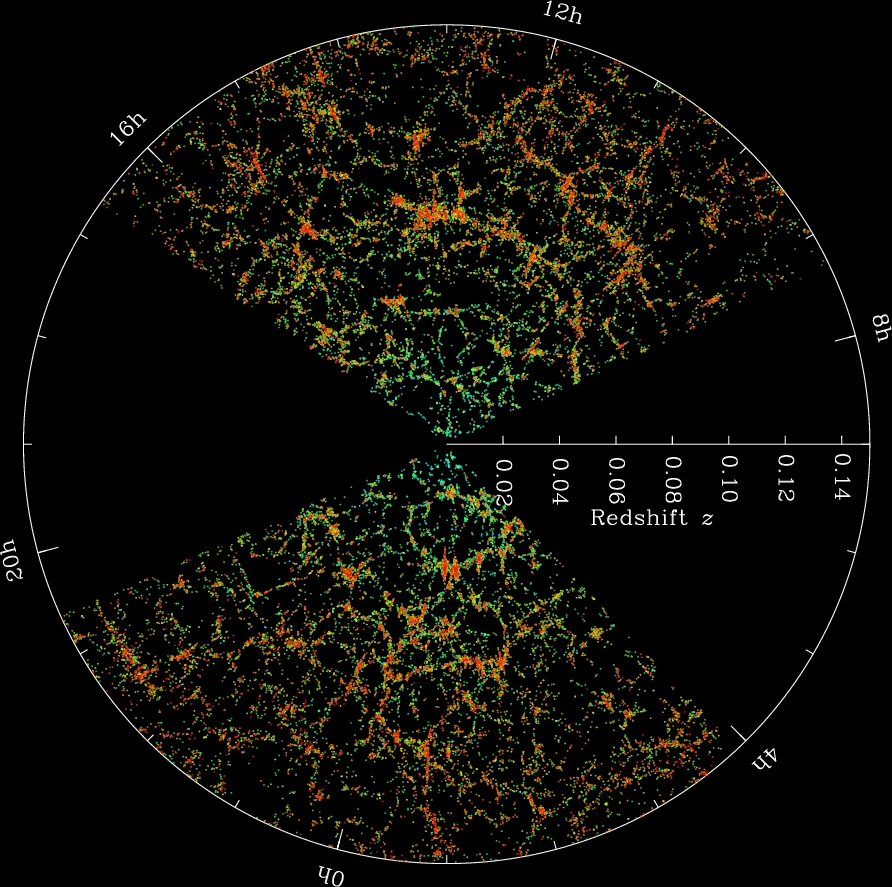
Sloan Digital Sky Survey
The Sloan Digital Sky Survey is a massive scientific undertaking to map objects of the known universe. Hundreds of millions of objects have been observed going back billions of years. It may seem overwhelming to even begin processing this data, but a simple map of the objects in the sky provides immediate insight into the large scale structure of our universe. We find that galaxies are bound by gravity to form massive filaments, and that these filaments must contain mass beyond what we can see (in the form of dark matter) to form these web-like structures.

Fingers of God

Fingers of God
If you plot galaxies to observe large-scale structure, a peculiar pattern emerges. The structures seem to point inward and outward from our position in the universe. This violates the Cosmological Principle, which states that no position in the universe should be favored over any other. So why do these filaments seem to point at us? The cause of these “Fingers of God” is an observational effect called redshift-space distortion. The galaxies are moving due to larger gravitational forces of their cluster, as well as the expansion of the universe, so their light seems to be accelerated towards or away from us. Correcting for this effect gives us the more random filaments we see above.

Expansion of the Universe

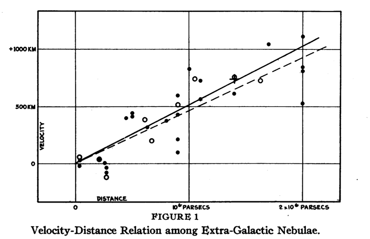
Hubble's Law
In 1929, Edwin Hubble published a simple yet revolutionary plot. He plotted the distance of galaxies from us, and the velocities at which they moved toward or away from us. What he found was that the farther away a galaxy was, the faster it moved away from us. This could not be the case in what was thought to be a static universe. Hubble’s Law came to prove that our universe was in fact expanding.

Galaxy Rotation Curves

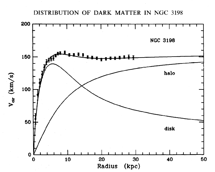
Rotation Curve of NGC3198
When we plot the rotational velocity of galaxies, we expect the rotational velocity to fall off as the radius increases based on the mass we can observe. As we get further away from the center and into less-dense regions, the matter should lose angular momentum and rotate slower. However, plotting rotational velocity curves reveals something peculiar — the rotational velocity remains constant regardless of radius as you leave the center. This means there must be matter we aren’t seeing: dark matter.

Our own research

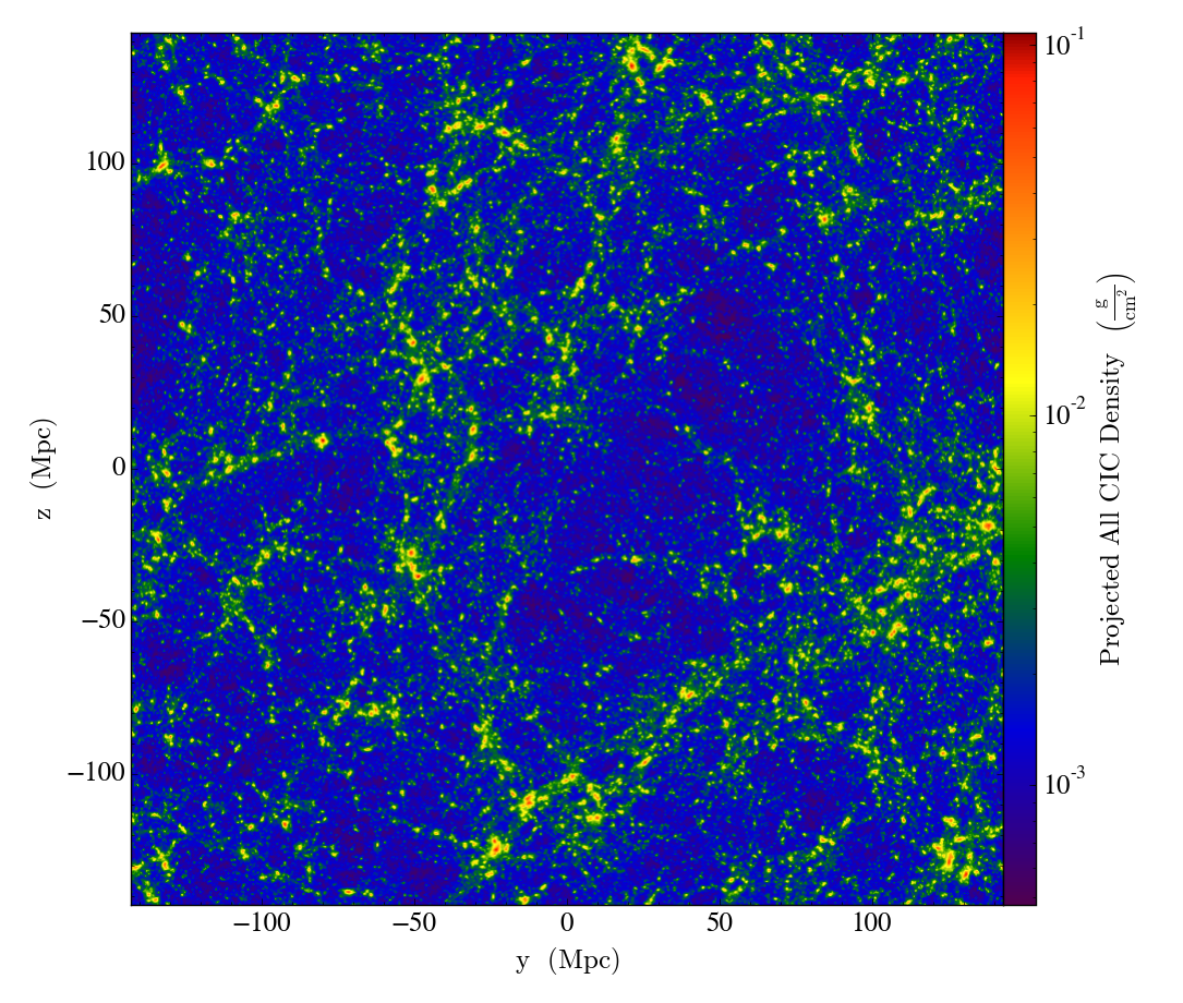
Density Plot
Visualization has proved important in our own research as well. Simple sanity checks on the large-scale structure of our simulations helps us make sure our simulations are running properly. Plots of different parameters show simple relationships that arise from the physics of our simulations.