PlaNet: Classifying Planets with Neural Networks

After completing Jeremy Howard’s Deep Learning course, I wanted to put my skills to the test on something fun and interesting, so I set out to train a neural network that classified planets. I’m happy with the end result (and its cheeky name): plaNet.

I wanted to classify major solar system planets based on salient features. The issue with this approach is that there isn’t very much data to train a neural network on. I scraped AstroBin for amateur photos of planets, but I found that most of them simply looked like smudges, and the outer planets were either unrecognizable or missing entirely.

Some of the unaugmented training data used for Jupiter, mostly from NASA.

To get around these issues, I based my approach on two methods: data augmentation on my small dataset, and fine-tuning an existing neural network. Data augmentation is simple in Keras, so I dramatically increased my dataset size simply by applying transformations to my initial images. I fine-tuned my network on VGG’s ImageNet convolutional layers (a classic approach to transfer learning). I dropped out the last fully-connected layer, which was trained to classify everyday objects, and kept the convolutional layers. These layers are great for identifying features — edges, shapes, and patterns — that could still be found in my images of planets. At this point, I pre-calculated the output of the convolutional layer on the initial and augmented datasets in order to easily combine them into one feature set, then I was able to train with a relatively solid test accuracy (~90%). I used a high dropout rate in order to avoid overfitting to my small training dataset, and it seems to have worked.

I want to highlight the simplicity of this approach. Because we’re simply fine-tuning a pre-trained neural network, we can access what is essentially the state of the art in deep learning with just a few lines of code and a small amount of computing time and power (compared to training an entire network from scratch). My work was mostly in preparing the datasets and fine-tuning different parameters until I was happy with the results. If you haven’t already, I encourage you to take a look at the course online. Many thanks to Jeremy Howard for giving me a practical approach to something I’ve only had theoretical backing for so far.
Sagan Exoplanet Workshop Day 1

Morning

Eric Feigelson (Penn State) discusses Statistics and the Astronomical Enterprise, and why statistics are so essential to the discovery and study of Exoplanets. The history and development of statistics in relation to astronomy as well as the present state of the field are covered. Key examples of essential statistical applications in astronomy and astrophysics are discussed, as well as an outlook on potential future developments and applications. Practical computing implementations with R are discussed.

Jessi Cisewski (Yale) goes over Bayesian Methods. She covers the basics of Bayesian analysis (Bayes’ Theorem, prior and posterior distributions, and inference with posteriors). Examples of different analyses using different models and distributions are given. Classical/Frequentist approaches are contrasted with the Bayesian approach, and best practices are covered.

Xavier Dumusque (Universite de Geneva) and Nikole Lewis (STScI) introduce the hands-on sessions of the week. Xavier discussed differentiating Radial Velocity signals from planetary signals, and Nikole discussed detecting exoplanets in upcoming JWST data and analyzing their spectra.

Afternoon

David Kipping (Columbia) gives A Beginner’s Guide to Monte Carlo Markov Chain (MCMC) Analysis. MCMC examples are covered as a way to find a posterior distribution. Metropolis and Metropolis-Hastings algorithms are discussed, and situations where other algorithms may be more or less effective are presented.

POPs Session I

Slides here.

  • Ines Juvan (Space Research Institute Graz) – PyTranSpot – A tool for combined transit and stellar spot light-curve modeling
  • Anthony Gai (Univ. at Albany) – Bayesian Model Testing of Models for Ellipsoidal Variation on Stars Due to Hot Jupiters
  • Emiliano Jofre (OAC-CONICET) – Searching for planets in southern stars via transit timing variations
  • Sean McCloat (Univ. of North Dakota) – Follow-up Observations of Recently Discovered Hot Jupiters
  • Romina Petrucci (OAC-CONICET) – A search for orbital decay in southern transiting planets
  • Luke Bouma (MIT) – What should we do next with the Transiting Exoplanet Survey Satellite?
  • Akshata Krishnamurthy (MIT) – A precision optical test bench to measure the absolute quantum efficiency of the Transiting Exoplanet Survey Satellite CCD detectors

David Kipping (Columbia) teaches us about using Bayesian Priors for Transits and RVs. Selection, implementation, strengths and weaknesses, and ideal use cases for different types of priors are discussed.

POPs Session II

Slides here.

  • Allen Davis (Yale) – Assessing the information content of spectra using PCA
  • Matteo Pinamonti (Univ. of Trieste) – Searching for planetary signals in Doppler time series: a performance evaluation of tools for periodogram analysis
  • Keara Wright (Univ. of Florida) – Stellar Parameters for FGK MARVELS Targets
  • Richard Hall (Univ. of Cambridge) – Measuring the Effective Pixel Positions of the HARPS3 CCD
  • Sarah Millholland (UCSC) – A Search for Non-Transiting Hot Jupiters with Transiting Super-Earth Companions
  • Tarun Kumar (Thapar Univ.) – Radial Velocity Curves of Polytropic Models of Stars of Polytropic Index N=1.5
  • Fei Dai (MIT) – The K2-ESPRINT Collaboration

Eric Feigelson (Penn State) covers Statistical Approaches to Exoplanetary Science. The talk focuses on time series analysis. Parametric and nonparametric methods are shown for time domain and frequency domain  problems. Code examples and other potentially useful methods are given.

dotAstronomy Day 1

James Webb Space Telescope and Astronomy

Sarah Kendrew (ESA, STScI)

JWST goes well into the infrared
Launch Autumn/winter 2018 — lots of things that can go wrong, but these engineers are awesome.
Science proposals start November 2017.
Routine science observations start six months after launch.
Compared to next-gen observatories, JWST is an old school telescope. We can bring it into the 21st century with better tools for research.
Coordination of development tools with Astropy developers.
Watch the clean room live on the WebbCam(ha!).

Bruno Merin (ESA)

ESASky – a Multi-Mission Interface

Open Source Hardware in Astronomy

Carl Ferkinhoff (Winona State University)

hardware.astronomy
Bringing the open hardware movement to astronomy
1) Develop low(er) cost astronomical instruments
2) Invest undergrads in the development (helps keep costs low).
3) Make hardware available to broader community
4) develop an open standard for hardware in astronomy

Citizen Science with the Zooniverse: turning data into discovery (Oxford)

Ali Swanson

Crowdsourcing has been proven effective at dealing with large, messy data in many cases across different fields.
Amateur consensus agrees with experts 97% of the time (experts agree with each other 98% of the time), and remaining 3% are deemed “impossible” even by experts.
Create your own zooniverse!

Gaffa tape and string: Professional hardware hacking (in astronomy)

James Gilbert (Oxford)

Spectra with fiber optic cables on a focal plane.
Move the cables to new locations.
Use a ring-magnet and piezoelectric movement to move “Starbugs” around — messy, inefficient.
Prototyped a vacuum solution that worked fine! This is now the final design.
Hacking/lean prototypes/live demos are effective in showing and proving results to people. Kinks can be ironed out later, but faith is won in showing something can work.

Open Science with K2

Geert Barentsen (NASA Ames)

Science is woefully underfunded.
Qatar World Cup ($220 billion) vs. Kepler mission ($0.6 billion)
Open science disseminates research and data to all levels of society.
We need more than a bunch of papers on the ArXiv.
Zooniverse promotes active participation.
K2 mission shows the impact of extreme openness.
Kepler contributed immensely to science, but it was closed.
Large missions are too valuable to give exclusively to the PI team — don’t build a wall.
Proprietary data slows down science, misses opportunities for limited-lifetime missions, blocks early-career researchers, and reduces diversity by favoring rich universities.
People are afraid of getting scooped, but we can have more than one paper.
Putting work on GitHub is publishing, and getting “scooped” is actually plagiarism.
K2 is basically a huge hack — using solar photon pressure to balance an axis after K1 broke.
Open approach: no proprietary data, funding other groups to do the same science, requires large programs to keep data open.
K2 vs K1: The broken spacecraft with a 5x smaller budget has more authors and most publications, and more are early-career researchers because all the data is open. 2x increase, and a more fair representation of the astro community.
Call to action: question restrictive policies and proprietary periods. Question the idea of one paper for the same dataset or discovery. Don’t fear each other as competition — fear losing public support.
The next mission will have open data from Day 0 thanks to K2.

Lightning Talks

#foundthem

Aleks Scholz (University of St Andrews)

SETI, closed science vs open science and communicating with the public.

astrobites

Ashley Villar (Harvard)

Send your undergrads to Astrobites! Advice, articles, tutorials.

There is no such thing as a stupid question comic book

Edward Gomez (Las Cumbres Observatory)

Neat astro comic book for kiddos.

Astronomy projects for the blind and visually impaired

Coleman Krawczyk (University of Portsmouth)

3D printing galaxies as a tool for the blind.

NOAO Data Lab

Matthew Graham (Caltech/NOAO)

Classifying Stellar Bubbles

Justyn Campbell-White (University of Kent)

Citizen science data being used in a PhD project.

The Pynterferometer

Adam Avison (ALMA)

A short history of JavaScript

William Roby (Caltech)

JavaScript is more usable thanks to ES6, and it follows functional principles. Give it another try if you’ve written it off!

Asteroid Day – June 30th, 2016

Edward Gomez (Las Cumbres Observatory)

International effort to observe NEAs with Las Cumbres.

The Importance of Data Visualization in Astronomy

It is difficult to understate the importance of data visualization in astronomy and astrophysics. Behind every great discovery, there is some simple visualization of the complex data that makes the science behind it seem obvious. As good at computers are becoming at making fits and finding patterns, the human eye and mind are still unparalleled when it comes to detecting interesting patterns in data to reach new conclusions. Here are a few of my favorite visualizations that simply illustrate complex concepts.

Large Scale Structure

As we’ve mapped increasing portions of the known universe, we’ve discovered astounding structures on the largest scales. Visualizing this structure in 2D or 3D maps gives us an intuitive grasp of the arrangement of galaxies within the universe and the forces the creation of that structure.

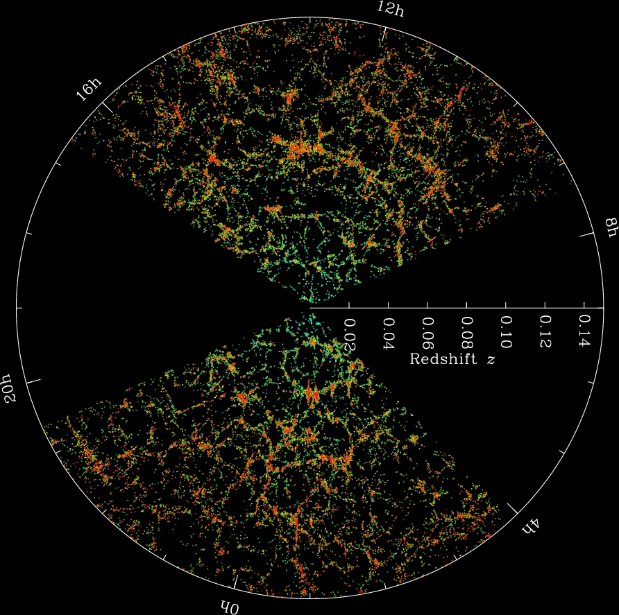
Galaxy filaments

Sloan Digital Sky Survey
The Sloan Digital Sky Survey is a massive scientific undertaking to map objects of the known universe. Hundreds of millions of objects have been observed going back billions of years. It may seem overwhelming to even begin processing this data, but a simple map of the objects in the sky provides immediate insight into the large scale structure of our universe. We find that galaxies are bound by gravity to form massive filaments, and that these filaments must contain mass beyond what we can see (in the form of dark matter) to form these web-like structures.

Fingers of God

Fingers of God
If you plot galaxies to observe large-scale structure, a peculiar pattern emerges. The structures seem to point inward and outward from our position in the universe. This violates the Cosmological Principle, which states that no position in the universe should be favored over any other. So why do these filaments seem to point at us? The cause of these “Fingers of God” is an observational effect called redshift-space distortion. The galaxies are moving due to larger gravitational forces of their cluster, as well as the expansion of the universe, so their light seems to be accelerated towards or away from us. Correcting for this effect gives us the more random filaments we see above.

Expansion of the Universe

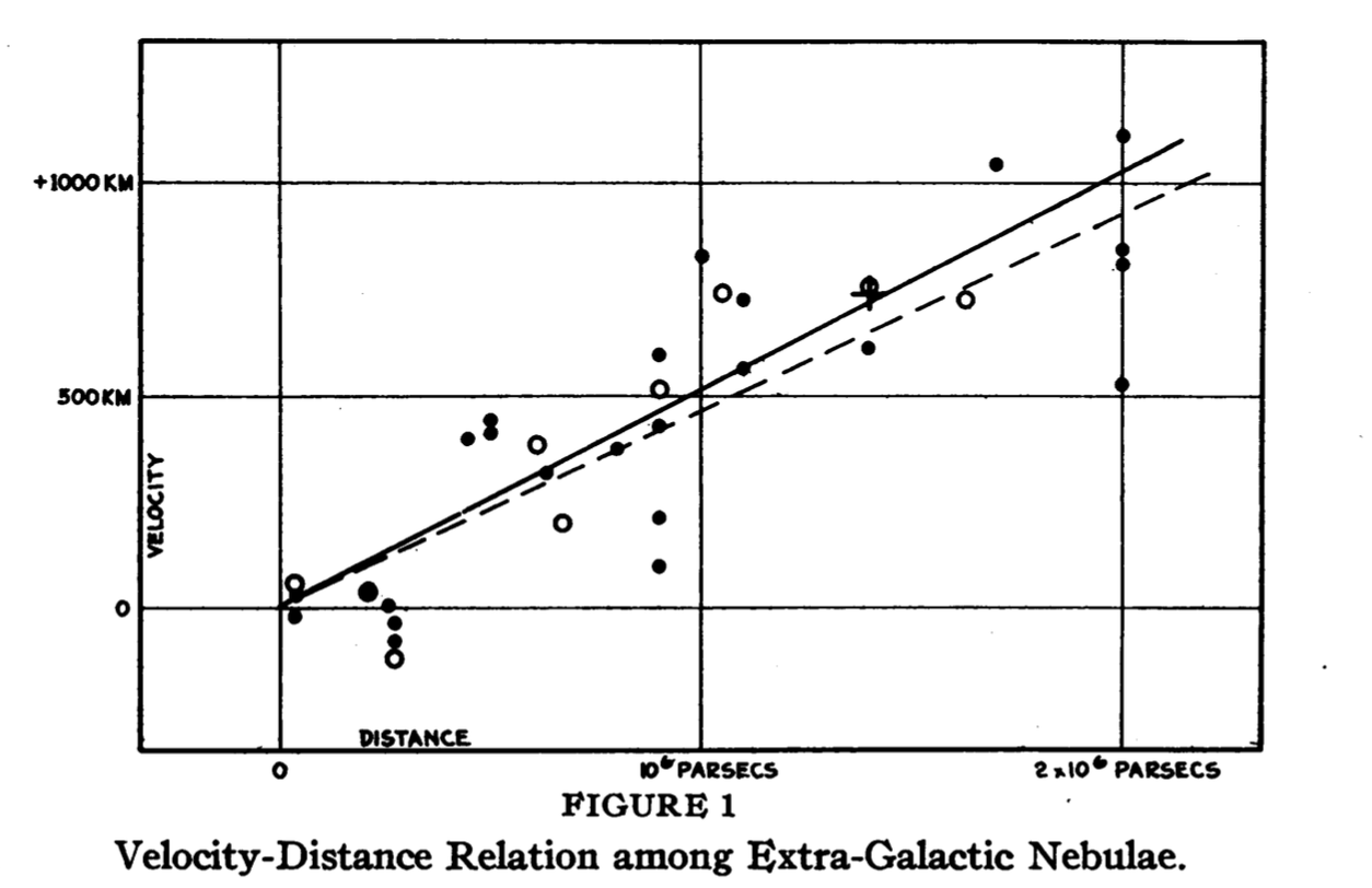
Hubble's Law
In 1929, Edwin Hubble published a simple yet revolutionary plot. He plotted the distance of galaxies from us, and the velocities at which they moved toward or away from us. What he found was that the farther away a galaxy was, the faster it moved away from us. This could not be the case in what was thought to be a static universe. Hubble’s Law came to prove that our universe was in fact expanding.

Galaxy Rotation Curves

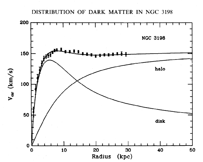
Rotation Curve of NGC3198
When we plot the rotational velocity of galaxies, we expect the rotational velocity to fall off as the radius increases based on the mass we can observe. As we get further away from the center and into less-dense regions, the matter should lose angular momentum and rotate slower. However, plotting rotational velocity curves reveals something peculiar — the rotational velocity remains constant regardless of radius as you leave the center. This means there must be matter we aren’t seeing: dark matter.

Our own research

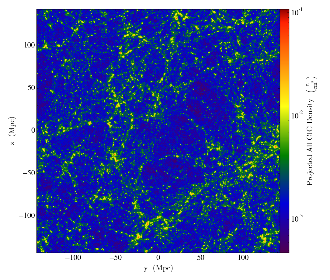
Density Plot
Visualization has proved important in our own research as well. Simple sanity checks on the large-scale structure of our simulations helps us make sure our simulations are running properly. Plots of different parameters show simple relationships that arise from the physics of our simulations.